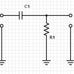
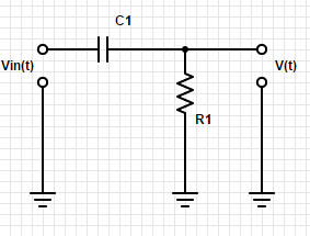
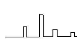
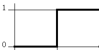
This is an example of a differentiator. Send a signal in, and the signal you get out will be just the edges of the wave form. If the input signal is a square wave, then the output will be a series of spikes at each of the sides of the square wave
Incidentally, having a wave that includes spikes could indicate that you have unintentional capacitive coupling.
Let’s look at how voltage (V) and current (I) change with respect to time in circuits with capacitors and resistors.
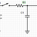
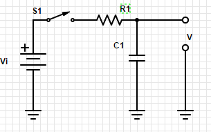
Take a look at this circuit:
Close the switch S1 connecting the capacitor (C1) to the battery (Vi) through resistor (R1). How fast will C1 charge?
That is determined by the relationship between R1 and C1. It is known as the RC time constant.
Assuming that C1 = 1 microfarad and R1 = 1k ohm, then the time constant will be 1. And we have a shortcut that it will be within 1% of the input voltage with in 5RC, so within 5 seconds.
Capacitors hold charge. Capacitors do not conduct.
We measure capacitance in farads and charge in coulombs (equivalent to the charge 6×10^18 electrons).
a capacitor with 1 farad of capacity will charge 1 coulomb of charge after 1 volt has been applied across its terminals for 1 second.
Q=CV
The capacitor is basically plates of two conductors separated by a non-conductor. When a voltage is applied, the charge accumulates. And when the voltage has been removed, then it can release that charge.
I found this really cute video that explains a capacitor:
The total capacitance of capacitors in parallel is the sum of the capacitors.
Ctotal = C1+C2+C3…
Capacitors in parallel will always result in a BIG capacitance.
However capacitors in series will always result in a smaller capacitance. Two capacitors in series have the capacitance of:
Ctotal = (C1C2)/(C1+C2)
Capacitors in series will always result in a capacitance smaller than the smaller capacitor.
Since capacitors do not conduct current, they do not dissipate power.
There are a variety of test equipment that can create signals with ranges of different characteristics. Three classes of these signal sources we will talk about today: Signal Generators, Pulse Generators, and function Generators.
Signal Generators produce sine waves while allowing you to define the amplitude, frequency, and even allowing for these to vary overtime.
Pulse Generators create pulses, allowing for you to vary the amplitude, pulse width, frequency, and even rise time and fall time.
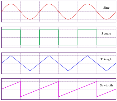
Function Generators allow for you to create more complex waves, in a variety of shapes:
Let’s cover two sections today:
1.09 Other signals
1.10 Logic Levels
We have been looking at Voltage as a function of time and seeing how it will look on a graph. The past few days we have talked about graphs that are sine wave.
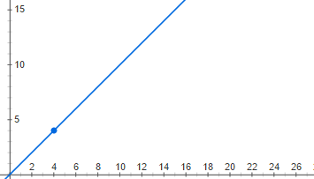
But there could be other ways that this could look too. Consider if voltage started out at zero and continued to increase. It would look something like this:
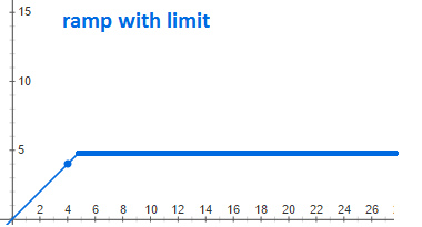
But it is not possible to increase voltage indefinitely and so the graph would really look like this: (Ramp with limit)
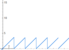
But there are other interesting graphs to. Consider the case of voltage increasing to a point, and then when it reaches a certain point it goes to zero and then begins again. Let’s say you have a circuit that triggers at a certain voltage, and a capacitor that you are charging up till that point. It might looks something like this sawtooth wave:
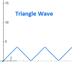
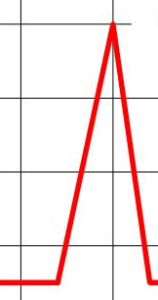
But you can also imagine a case where it reaches a point and decreases at the same linear rate. This would look like a triangle wave:
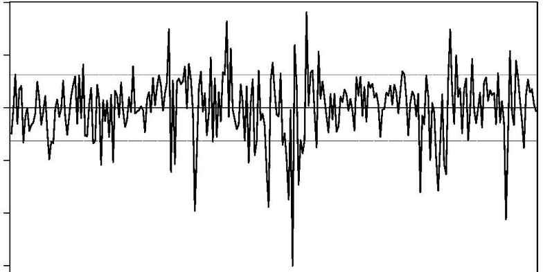
And then there is noise, a complex, background static that we always need to consider and usually minimize:
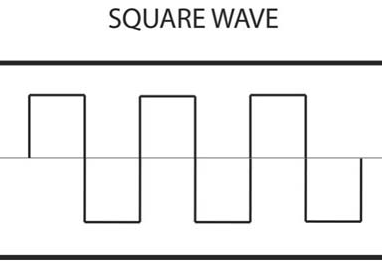
Square waves
Steps
Spikes
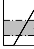
But in digital electronics we concern ourselves with logic levels and interrupting a particular voltage as either a true or a false; as a on or a off; as a 1 or 0. Most digital electronics have a threshold voltage. Above that voltage it is considered to be true/on/1. Below that voltage it is considered to be false/off/0.
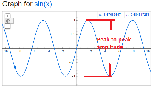
Peak-to-peak amplitude (pp amplitude) is twice the amplitude. This is the measurement of the amplitude from the bottom peak to the top peak as illustrated below:
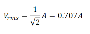
root-mean-square amplitude (rms amplitude) has different formulas based upon the shape of the signal. For sine waves only it is given by:
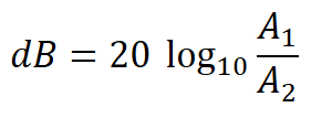
Decibels is a comparison between two signals.
When comparing amplitude use this formula:
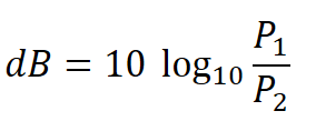
When comparing the power use this formula:
Sometimes decibels are presented as units. This is because their is an implicit signal that is being used for comparison. Here are some common ones:
a) dBV: 1 volt rms
b) dBm – the voltage corresponding to 1mW with an assumed load impedance
c) small noise generated by a resistor at room temperature
The next few sections in The Arts of Electronics deals with signals. What are the characteristics of signals? Amplitude, frequency, shape, etc.
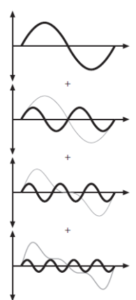
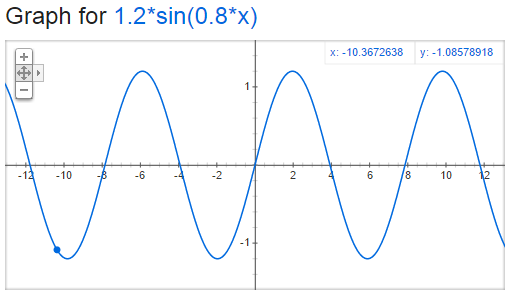
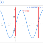
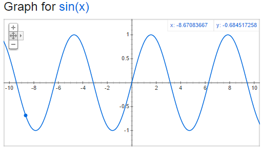
The values we are looking at is voltage as a function of time. The most basic signal is the sinusoidal signal. Have you ever graphed y=sin(x) and end up with:
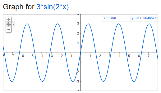
But how would you compare this wave to the following:
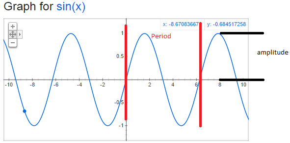
There are two key things to think about when comparing sine waves: frequency and amplitude. The amplitude is the distance from y=0 to the top of the sine wave. The frequency is how many times the wave repeats in a given period of time. We typically use the unit hertz (Hz) for frequency, which is one cycle (or period) per second. Lets take a look at period and amplitude in our original sine graph:
The formula that you should remember is
V=A*sin(2*pi*f*t)
A is the amplitude in volts, f is the frequency in Hz and t is the time in seconds.
Ohm’s law is R=V/I. For the ordinary resistance, this is a constant proportion for a large range of V. But this is not true for all devices. Today we look at the Zener diode which has a high resistance up to a point and then almost no resistance for a large range of V. Also, we look at the tunnel diode (also known as the Esaki diode) which actually has a negative resistance over a particular range of V.
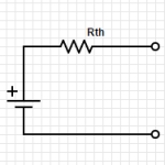
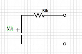
Any two terminal network of voltage sources and resistors can be replace by a single voltage source in combination with a single resistor. This is called the Thevenin’s equivalent circuit:
The first step is to identify the two terminals of the network.
Then to figure out Rth, replace any voltage sources with short circuits and any current sources with open circuits.
Calculate the voltage between the two terminals.
Then figure out Vth between the two terminals.
To figure this out using testing and measuring, it is only necessary to find the voltage at the two terminals with power on, and the resistance with power off.
This can greatly simplify circuit analysis of complex circuits.
Check out videos on YouTube with more detailed information:
Let’s take a look at the symbols for voltage sources and current sources. Also, let’s discuss the properties of the ideal voltage source and the ideal current source.
The ideal voltage source will maintain the same voltage between its terminals regardless of the load. This is easiest with an open circuit but becomes impossible with a short circuit.
The ideal current source will maintain the same current regardless of the resistance of the load. This is easy with an open circuit but becomes more and more difficult as the resistance increases.